Operational amplifier (op-amp) is an electronic device with two input terminals and a single output terminal. It is a fundamental building block of analog circuits, widely used for signal amplification, voltage comparison, filtering, buffering, and mathematical operations.
The Basics of the Operational Amplifier
In this operational amplifier basics guide, we will explore the working principles and important characteristics of op-amps. An operational amplifier is a high-gain electronic device commonly used for signal amplification, conditioning, filtering, and analog mathematical operations such as addition, subtraction, integration, and differentiation.
An operational amplifier (op-amp) is primarily a voltage amplifier designed to operate with external components such as resistors and capacitors. These components are connected around the op-amp to provide feedback, which determines how the circuit behaves and what function it performs.
By changing the feedback network, an op-amp can be configured for different applications. Depending on whether the feedback components are resistive, capacitive, or a combination of both, the same basic device can perform a wide range of analog signal-processing functions. This versatility is the reason it is called an operational amplifier.
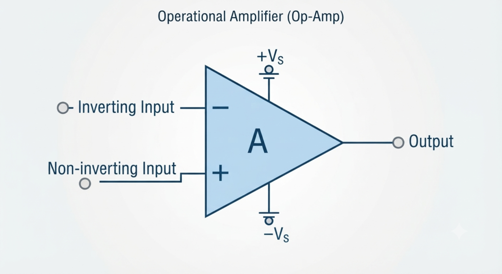
A typical op-amp has three main terminals: two high-impedance input terminals and one output terminal. The first input is the inverting input, identified by a minus sign (−), while the second is the non-inverting input, identified by a plus sign (+).
The third terminal is the output, which can source or sink current to the connected circuit within the device’s operating limits. For a linear op-amp, the output voltage is related to the differential input voltage and the amplifier’s gain. Depending on the type of input and output signals being considered, amplifier gain can be classified into different categories.
Operational Amplifier Basics of Classification
Operational amplifiers and related amplifier circuits can be classified according to the type of input and output signals they handle:
| Amplifier Type | Input | Output |
| Voltage Amplifier | Voltage | Voltage |
| Current Amplifier | Current | Current |
| Transconductance Amplifier | Voltage | Current |
| Transresistance Amplifier | Current | Voltage |
In most practical operational amplifier circuits, the op-amp is used as a voltage amplifier, where an input voltage produces a corresponding output voltage . Therefore, the following discussion focuses primarily on voltage-amplifier configurations.
An op-amp responds to the voltage difference between its two input terminals. Its input stage is essentially a differential amplifier, allowing the device to amplify the difference between the non-inverting and inverting input signals. The resulting differential input voltage determines the output response of the operational amplifier.
Operational Amplifier Basics – The Differential Pair
A differential amplifier is the fundamental input stage of a typical operational amplifier. It is designed to respond primarily to the voltage difference between two input signals. A basic differential pair uses two closely matched transistors, and , with their emitters connected together and biased through a common emitter resistor .
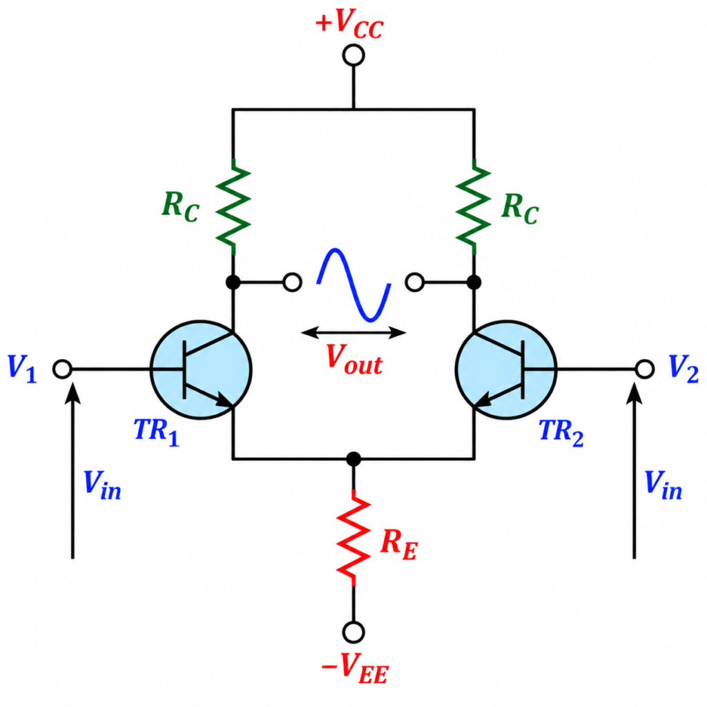
The two input signals, and , are applied to the transistor bases. When the voltage at one input increases, the corresponding transistor conducts more current while the other transistor conducts less. This complementary action allows the circuit to amplify the difference between the two input voltages.
Differential Amplifier and Common-Mode Operation
The differential pair is typically operated from a dual power supply, such as and . For closely matched transistors, changes in the individual collector currents tend to balance each other, providing stable differential operation.
The amplifier can operate in two important modes: differential mode and common-mode. In differential mode, the two input voltages are different, and the circuit amplifies their difference. In common-mode operation, the same signal is applied to both inputs. An ideal op-amp should reject this common signal and produce no corresponding change at its output.
The ability of an operational amplifier to reject common-mode signals is expressed by its Common-Mode Rejection Ratio (CMRR). A higher CMRR indicates better rejection of signals that appear simultaneously at both inputs.
A practical operational amplifier has a very high open-loop differential gain, represented by . Open-loop operation means that no external feedback path is connected between the output and input. Because the open-loop gain is extremely high, even a small differential input voltage can produce a large output voltage.
In practical circuits, negative feedback is normally applied to control the overall closed-loop gain. The feedback network allows the amplifier to achieve a stable and predictable gain determined primarily by the external components.
Thus, the fundamental operation of an op-amp can be understood from its differential input stage: it responds to the difference between the voltages at its two input terminals, rather than simply to their common voltage level. The relationship between this differential input and the output is described by the open-loop differential gain .
Equivalent Circuit of an Ideal Operational Amplifier
An ideal operational amplifier can be represented by a simple equivalent model with two high-impedance input terminals and one low-impedance output terminal. The model assumes perfect characteristics that simplify the analysis and design of op-amp circuits.
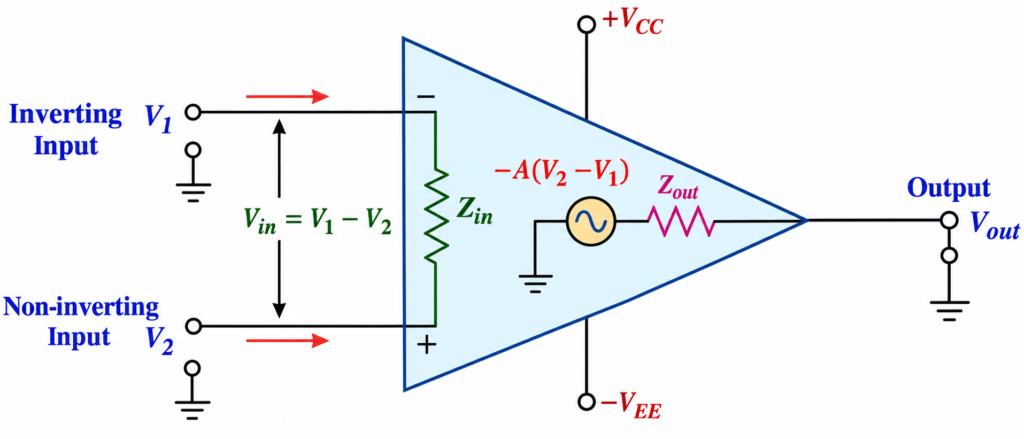
Op-amp Parameters and Idealised Characteristics
The main ideal characteristics of an operational amplifier are summarized below:
| Parameter | Ideal Value | Description |
| Open-loop gain, AVO | Infinite | An ideal op-amp provides unlimited voltage amplification without external feedback. |
| Input impedance, ZIN | Infinite | No current flows into either input terminal. |
| Output impedance, ZOUT | Zero | The output behaves like an ideal voltage source and can deliver voltage to the load without an internal voltage drop. |
| Bandwidth, BW | Infinite | An ideal op-amp can amplify signals over an unlimited frequency range. |
| Input offset voltage, VIO | Zero | The output is zero when the differential voltage between the two inputs is zero. |
Ideal Op-amp Rules
These ideal characteristics lead to two important assumptions used when analysing operational amplifier circuits.
Current rule: Since the input impedance is infinite, no current flows into the inverting or non-inverting input terminals:
Voltage rule: When an ideal op-amp operates with negative feedback in its linear region, the voltage difference between its two input terminals approaches zero:
These two assumptions greatly simplify the analysis of common op-amp circuits, including inverting amplifiers, non-inverting amplifiers, voltage followers, and summing amplifiers.
Practical Operational Amplifier Characteristics
Real operational amplifiers do not have infinite gain, infinite bandwidth, or zero output impedance. Their performance is limited by the internal design of the device. For example, the µA741 is an older general-purpose op-amp whose open-loop gain is very high at low frequencies but decreases as frequency increases.
This reduction in gain with frequency is an important characteristic of practical op-amps. The gain-bandwidth product (GBW) describes the relationship between an op-amp’s open-loop gain and its usable frequency range. As the operating frequency increases, the available open-loop gain decreases until it approaches unity.
Real op-amps also have finite input impedance, non-zero output impedance, input offset voltage, input bias current, and limited output current. Therefore, the ideal model is primarily used to understand circuit operation, while the manufacturer’s datasheet should be consulted when analysing a practical op-amp circuit.
Operational Amplifier Basics – Open-Loop Frequency Response
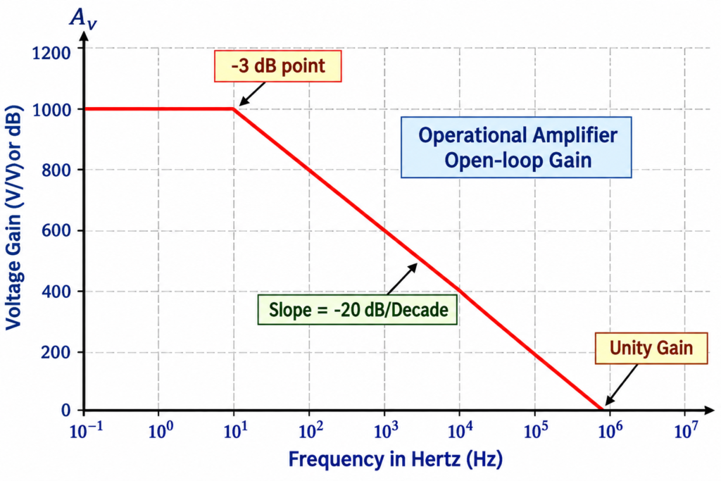
The open-loop frequency response of an operational amplifier shows how its voltage gain changes as the operating frequency increases. For a typical op-amp, the open-loop gain is very high at low frequencies and gradually decreases as frequency rises.
Over the amplifier’s dominant frequency range, the product of voltage gain and frequency remains approximately constant. This relationship is known as the Gain-Bandwidth Product (GBP) or Gain-Bandwidth Product (GBW).
The relationship can be written as:
For example, if the open-loop gain at 100 kHz is 20 dB, the corresponding voltage gain is 10. Therefore:
At 1 kHz, if the amplifier has a gain of 60 dB, its voltage gain is 1,000. The gain-bandwidth product is then:
Both calculations produce approximately the same value, illustrating the constant gain-bandwidth relationship within the applicable frequency range.
The voltage gain of an operational amplifier can be calculated from the ratio of the output voltage to the input voltage:
For expressing voltage gain in decibels (dB), the logarithmic relationship is used:
The open-loop frequency response is important because it explains why an op-amp cannot maintain its maximum open-loop gain at all frequencies. As frequency increases, the available gain falls, which also limits the bandwidth of practical op-amp circuits.
An Operational Amplifier’s Bandwidth
The bandwidth of an operational amplifier is the range of frequencies over which it can operate while maintaining its specified voltage gain. The upper cutoff frequency is commonly defined at the −3 dB point, where the voltage gain falls to approximately 70.7% of its maximum value.
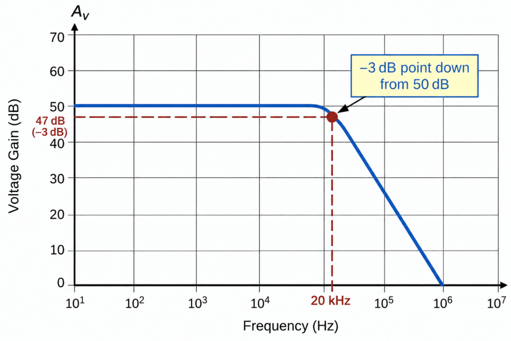
At the −3 dB frequency, the output voltage has decreased to about 0.707 of its low-frequency value. As the frequency increases beyond this point, the amplifier’s voltage gain continues to decrease.
For example, consider an operational amplifier with a low-frequency gain of 50 dB. At the −3 dB point, the gain falls to approximately 47 dB. If the amplifier has a gain-bandwidth product (GBP) of 2 MHz, the corresponding cutoff frequency can be determined from the gain-bandwidth relationship.
This calculation provides a more accurate value for the amplifier’s bandwidth than estimating the cutoff frequency directly from the frequency-response graph.
Operational Amplifier Worked Example No. 1
Using the voltage-gain relationship in decibels, we can determine the amplifier gain at the −3 dB point:
Therefore,
The bandwidth can then be calculated using the gain-bandwidth product:
For a gain-bandwidth product of 2 MHz:
Therefore, the bandwidth of the amplifier at a gain of 50 dB is approximately 8.93 kHz. This value represents the frequency at which the gain falls by 3 dB from its maximum value.
Operational Amplifier Worked Example No. 2
Now consider what happens when the closed-loop gain of an operational amplifier is reduced. For a constant gain-bandwidth product, reducing the gain allows the amplifier to operate over a wider frequency range.
For example, if the amplifier gain is reduced to 30 dB, the corresponding bandwidth will increase compared with the bandwidth at a higher gain. This demonstrates the fundamental relationship between amplifier gain and bandwidth: as gain decreases, bandwidth increases, and vice versa.
The −3 dB frequency is particularly important because it represents the point where the output voltage falls to approximately 70.7% of its maximum value. Since power is proportional to the square of voltage, the output power at this frequency becomes approximately half of its maximum value.
At the or point:
Therefore:
Thus, the −3 dB corner frequency is also known as the half-power point, because the output power is approximately 50% of its maximum value at this frequency.
Types of Op-Amps
Operational amplifiers are versatile building blocks used in a wide range of linear and nonlinear analog circuits. Different op-amp configurations are designed to perform specific functions, from amplifying small differential signals to providing accurate signal conditioning and power amplification.
Some common types and configurations include:
- Differential Amplifier: Amplifies the voltage difference between two input signals while rejecting signals common to both inputs.
- Instrumentation Amplifier: Typically uses multiple op-amp stages to provide accurate amplification of low-level signals from sensors and transducers. It offers high input impedance and good common-mode rejection.
- Isolation Amplifier: Provides electrical isolation between the input and output sections while transferring an analog signal. It is useful when the two circuits must operate at different voltage potentials.
- Negative-Feedback Amplifier: Uses an op-amp with an external feedback network to control the closed-loop gain, improve stability, and provide predictable circuit performance.
- Power Amplifier: Designed to deliver higher current and power to a load. Power amplifier stages are commonly used when a small input signal must drive a relatively demanding load.
Operational Amplifier Configurations
Two primary configurations for operational amplifiers, or op-amps, are open-loop and closed-loop. The op-amp amplifies and processes the input signal in accordance with these arrangements.
Open-Loop Configuration
There is no feedback between the input and the output in an open-loop setup. At its highest gain, the op-amp functions at a very high level (usually in the region of 100,000 or more).
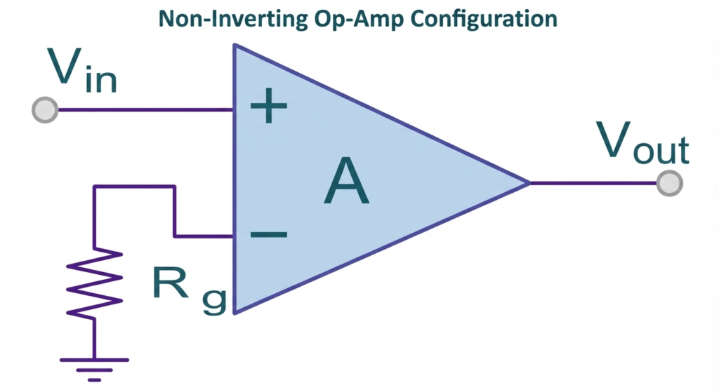
However, this results in a very sensitive amplifier that frequently experiences output saturation. Because they lack stability and control, open-loop systems are typically impractical for linear applications.
Key Features:
- Maximum gain.
- No feedback is used.
- Suitable for comparator applications where the output toggles between high and low states.
Closed-Loop Configuration
In a closed-loop system, some of the output is returned back into the system as positive or negative feedback (negative feedback is most prevalent). An op-amp with regulated output will behave predictably due to negative feedback, which aids in gain stabilization and control.
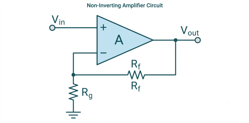
There are two types of closed-loop configurations:
- Inverting Configuration: The non-inverting terminal is grounded, and the input signal is connected to the inverting terminal. With a 180-degree phase shift from the input, the output is inverted.
- Non-Inverting Configuration: The non-inverting terminal receives the input signal. The output is regulated amplification of the input signal.
Key Features:
- Controlled and stable gain.
- Negative feedback improves linearity and reduces distortion.
- Commonly used in amplifiers, filters, and other signal processing circuits.
Real vs Ideal Op-Amp
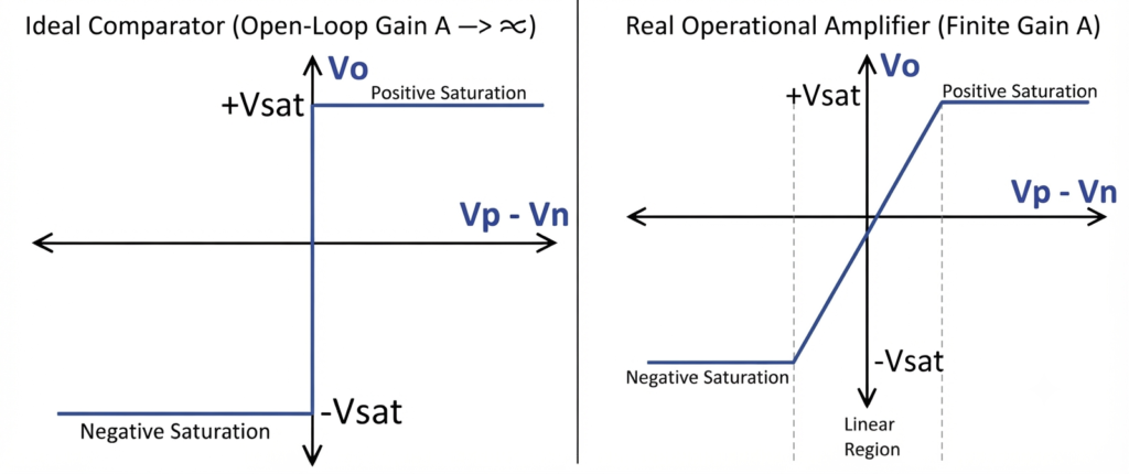
An ideal operational amplifier is a theoretical model with perfect characteristics, while a real op-amp has finite gain, bandwidth, and input/output impedances. Comparing these characteristics helps explain the practical limitations of op-amp circuits.
| Parameter | Ideal Op-Amp | Real Op-Amp |
| Voltage Gain | ∞ (Infinity) | Typically 10,000 to 100,000, depending on the device |
| Input Impedance | ∞ (Infinity) | Very high, commonly in the megaohm range or higher |
| Output Impedance | 0 Ω (Zero) | Low, but not zero |
| Bandwidth | ∞ (Infinity) | Limited and related to the gain-bandwidth product |
| Power Consumption | 0 W (Zero) | Depends on the specific op-amp and operating conditions |
| Input Offset Voltage | 0 V | Small, non-zero voltage |
| Input Offset Current | 0 A | Small difference between the two input bias currents |
| Input Bias Current | 0 A | Small current flowing into the input terminals |
| Input Capacitance | 0 F | Small parasitic capacitance at the input |
| Slew Rate | ∞ V/µs | Finite and specified by the op-amp manufacturer |
These differences are important when moving from ideal op-amp analysis to practical circuit design. Real devices also have limitations such as input offset voltage, input bias current, finite slew rate, and output current capability.
Operational Amplifier (Op-Amp) Classification Based on Supply
Operational amplifiers can also be classified according to their power-supply arrangement and input/output voltage range. Three common categories are dual-supply, single-supply, and rail-to-rail op-amps.
Dual-Supply Op-Amp
A dual-supply operational amplifier operates from separate positive and negative supply voltages, commonly represented as and . This arrangement provides a reference around 0 V and allows the output to swing in both positive and negative directions.
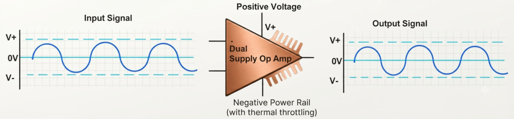
Dual-supply op-amps are commonly used in traditional analog circuits, audio systems, signal-conditioning circuits, and applications requiring bipolar signal amplification.
Single-Supply Op-Amp
A single-supply operational amplifier operates from one positive supply voltage with ground serving as the reference, such as and 0 V. This configuration is particularly useful in battery-powered, portable, and low-voltage electronic systems.

Because the supply does not extend below ground, the input and output signals may need appropriate biasing or level shifting to keep the op-amp within its allowable operating range.
Rail-to-Rail Op-Amp
A rail-to-rail operational amplifier is designed to operate with input and/or output voltages that can approach the positive and negative supply rails. This allows the device to make better use of the available supply-voltage range, particularly in low-voltage and battery-powered applications.
Depending on the device, rail-to-rail operation may apply to the input, output, or both. The exact voltage range should always be checked in the manufacturer’s datasheet.
Operational Amplifier Applications
An operational amplifier (op-amp) is a versatile building block used in both linear and nonlinear analog circuits. By combining an op-amp with external resistors, capacitors, and other components, many useful signal-processing and control functions can be implemented.
Linear Applications of Operational Amplifiers
In linear applications, the output changes predictably with the input, generally following a linear relationship. Common applications include:
- Adder (Summing Amplifier) – Combines two or more input voltages to produce a single output.
- Subtractor (Difference Amplifier) – Produces an output proportional to the difference between input voltages.
- Voltage-to-Current Converter – Converts an input voltage into a proportional output current; also called a transconductance amplifier.
- Current-to-Voltage Converter – Converts an input current into a proportional output voltage; also called a transresistance amplifier.
- Instrumentation Amplifier – Provides accurate amplification of small differential signals with high input impedance and good common-mode rejection.
- Power Amplifier – Provides increased current or power drive for loads requiring greater output capability.
Nonlinear Applications of Operational Amplifiers
Op-amps can also be used in circuits where the relationship between input and output is intentionally nonlinear. Examples include:
- Precision Rectifier – Rectifies low-level signals while minimizing the forward-voltage limitation of ordinary diodes.
- Peak Detector – Detects and holds the maximum value of an input signal.
- Clipper – Limits a signal to a specified voltage range.
- Clamper – Shifts the DC level of an AC waveform without significantly changing its shape.
- Sample-and-Hold Circuit – Samples an analog signal and holds its voltage for a defined period.
- Logarithmic and Antilogarithmic Amplifier – Performs logarithmic or exponential signal processing.
- Analog Multiplier and Divider – Performs multiplication or division of analog signals using suitable nonlinear circuitry.
- Comparator – Compares two input voltages and produces an output indicating which input is higher.
These applications demonstrate why the operational amplifier is widely used in analog signal processing, measurement, instrumentation, control, and electronic system design.
Conclusion
Hopefully by now we understand that on its own, an operational amplifiers is a very high gain DC differential amplifier which requires one or more external feedback networks or loops to control its voltage gain, frequency response and other such electrical characteristics.
We can connect external resistors and/or capacitors externally around an operational amplifier in a number of different ways to form basic Op-amp building block circuits such as: Inverting, Non-Inverting, Voltage Follower, Summing, Differential, Integrator and Differentiator type voltage amplifiers.
An “ideal” or perfect operational amplifier is a device with certain special characteristics such as infinite open-loop gain AO, infinite input resistance RIN, zero output resistance ROUT, infinite bandwidth 0 to ∞ and zero offset (the output is exactly zero when the input is zero).
There are a very large number of operational amplifier IC’s available to suit every possible application from standard bipolar, precision, high-speed, low-noise, high-voltage, etc, in either standard configuration or with internal Junction-FET transistors.
Operational amplifiers are available in IC dual-in-line packages consisting of either one single, dual or quad op-amp chips within one single device. The most commonly available and used of all the operational amplifiers in basic electronic kits and projects is the industry standard μA741.
The μA741 device is a general-purpose operational amplifier ideal to learn more about operational amplifier basics and the different types of circuit configurations you can construct using the μA-741.
Read Next: