Op Amp Characteristics: 7 Important Parameters Explained

Op amp characteristics describe the electrical properties and performance parameters of an operational amplifier. These characteristics determine how accurately an op amp amplifies input signals, responds to different frequencies, handles external loads, and rejects unwanted electrical noise.

An operational amplifier (op amp) is a high-gain voltage amplifier with two input terminals and one output terminal. The two inputs are called the inverting input and non-inverting input. It generally operates with a dual or single DC power supply and uses external components, such as resistors and capacitors, to perform different mathematical and signal-processing operations.

The main characteristics of an op amp include open-loop voltage gain, input impedance, output impedance, bandwidth, input offset voltage, and common-mode rejection ratio (CMRR).

These parameters are generally studied by comparing an ideal operational amplifier with a practical op amp. Understanding them helps in selecting the right operational amplifier for applications such as amplifiers, filters, oscillators, comparators, and signal-conditioning circuits.

Table of Contents

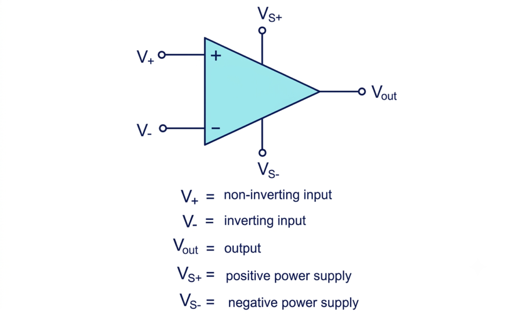
Op Amp Characteristics

The following table summarizes the six important characteristics of an operational amplifier and their ideal values.

Op Amp Characteristics	Ideal Op Amp	Practical Op Amp
Open-loop voltage gain	Infinite	Very high but finite
Input impedance	Infinite	High
Output impedance	Zero	Low but non-zero
Bandwidth	Infinite	Limited
Input offset voltage	Zero	Small non-zero value
Common-mode rejection ratio (CMRR)	Infinite	High but finite

Let’s understand each of these op amp characteristics in detail.

1. Open-Loop Voltage Gain (A)

Open-loop voltage gain is the ratio of the output voltage to the differential input voltage when an operational amplifier operates without external feedback.

It indicates how effectively an op amp amplifies the voltage difference between its inverting and non-inverting input terminals.

The open-loop voltage gain is expressed as:

A=\frac{V_{out}}{V_+-V_-}

Therefore, the output voltage is:

V_{out}=A(V_+-V_-)

Where:

$A$ = Open-loop voltage gain
$V_{out}$ = Output voltage
$V_+$ = Non-inverting input voltage
$V_-$ = Inverting input voltage

For an ideal operational amplifier, the open-loop voltage gain is infinite. This means that even an extremely small difference between the two input voltages can theoretically produce a large output voltage.

In a practical op amp, the open-loop voltage gain is very high but finite. Depending on the device, it may range from tens of thousands to several hundred thousand or more at low frequencies.

Example: If an op amp has an open-loop voltage gain of 100,000 and a differential input voltage of 100 µV, its theoretical output voltage is:

V_{out}=100000\times100\times10^{-6}

V_{out}=10V

The actual output is limited by the available power supply voltage and output swing.

2. Input Impedance (Zin)

Input impedance is the opposition offered by an operational amplifier to the current entering its input terminals. It determines how much current the op amp draws from the preceding circuit.

Input impedance is expressed as the ratio of the input voltage to the input current:

Z_{in}=\frac{V_{in}}{I_{in}}

Where:

$Z_{in}$ = Input impedance
$V_{in}$ = Input voltage
$I_{in}$ = Input current

The input impedance of an ideal op amp is infinite. Therefore, no current flows into its input terminals.

In a practical operational amplifier, the input impedance is high but finite. Its value depends on the input transistor technology and internal circuit design.

For example, CMOS and JFET-input op amps generally offer very high input impedance and low input bias current. Bipolar-input op amps typically have higher input bias current.

High input impedance is desirable because it minimizes the loading effect on the signal source.

3. Output Impedance (Zout)

Output impedance is the internal opposition offered by an operational amplifier to the current delivered to an external load.

It determines how effectively the op amp maintains its output voltage when the load current changes.

For a simplified output model, output impedance can be expressed as:

Z_{out}=\frac{\Delta V_{out}}{\Delta I_{out}}

Where:

$Z_{out}$ = Output impedance
$\Delta V_{out}$ = Change in output voltage
$\Delta I_{out}$ = Change in output current

An ideal operational amplifier has zero output impedance. It can maintain a constant output voltage regardless of the load current, within the ideal model.

A practical op amp has a small but non-zero output impedance. Its open-loop output impedance is generally higher than its closed-loop output impedance.

When negative feedback is applied, the effective output impedance is reduced. This improves the ability of the op amp to drive a load while maintaining a stable output voltage.

However, a practical op amp has limitations on its maximum output current and voltage swing.

4. Bandwidth (BW)

Bandwidth is the range of frequencies over which an operational amplifier can amplify an input signal effectively.

It determines how fast an op amp can respond to changes in the input signal without significant loss of gain.

An ideal op amp has infinite bandwidth. Therefore, its amplification capability remains unchanged at all frequencies, from DC to infinitely high frequencies.

A practical operational amplifier has limited bandwidth because of internal capacitances, frequency compensation, and other circuit characteristics.

The bandwidth of an op amp is commonly related to its gain-bandwidth product (GBW).

For a typical internally compensated op amp with a dominant-pole response:

GBW=A_{CL}\times BW

Where:

$GBW$ = Gain-bandwidth product
$A_{CL}$ = Closed-loop voltage gain
$BW$ = Closed-loop bandwidth

Example: Consider an op amp with a gain-bandwidth product of 1 MHz. If it operates with a closed-loop voltage gain of 10, its approximate bandwidth is:

BW=\frac{GBW}{A_{CL}}

BW=\frac{1MHz}{10}

BW=100kHz

This relationship is an approximation for a typical single-pole compensated op amp. Actual bandwidth depends on the device and circuit configuration.

5. Input Offset Voltage (Vio)

Input offset voltage is the small differential DC voltage that must be applied between the two input terminals of an operational amplifier to make its output voltage zero.

In an ideal op amp, the input offset voltage is zero. When both input terminals are at the same voltage, the output is ideally zero.

In a practical op amp, small mismatches in internal transistors and other circuit components produce an offset voltage. As a result, the output may not be exactly zero even when both inputs are connected to the same voltage.

Input offset voltage is usually specified in microvolts (µV) or millivolts (mV) in the manufacturer’s datasheet.

A lower input offset voltage is particularly important in precision applications, such as:

Instrumentation amplifiers
Temperature measurement circuits
Sensor signal conditioning
Medical measurement equipment
Low-level signal amplification

The input offset voltage may also change with temperature and time. This variation is known as offset voltage drift.

6. Common-Mode Rejection Ratio (CMRR)

Common-mode rejection ratio (CMRR) is the ability of an operational amplifier to reject signals that appear simultaneously and equally at both input terminals.

When the same voltage is applied to the inverting and non-inverting inputs, it is called a common-mode signal.

Ideally, an op amp amplifies only the difference between its two input voltages and completely rejects the common-mode component.

CMRR is defined as the ratio of differential voltage gain to common-mode voltage gain.

Mathematically:

CMRR=\frac{A_D}{A_{CM}}

Where:

$A_D$ = Differential voltage gain
$A_{CM}$ = Common-mode voltage gain

CMRR is generally expressed in decibels (dB):

CMRR(dB)=20\log_{10} \left(\frac{A_D}{A_{CM}}\right)

For an ideal operational amplifier, the common-mode gain is zero. Therefore, its CMRR is infinite.

A practical op amp has a finite CMRR, which means it cannot completely eliminate common-mode signals.

A higher CMRR indicates better rejection of unwanted signals, such as electrical noise and interference, that are common to both input terminals.

Example: Suppose an operational amplifier has a differential gain of 100,000 and a common-mode gain of 0.01.

CMRR=\frac{100000}{0.01}

CMRR=\frac{100000}{0.01}

In decibels:

CMRR(dB)=20\log_{10}(10^7)

CMRR=140,dB

Therefore, the CMRR of the operational amplifier is 140 dB.

A high CMRR is especially useful in instrumentation amplifiers, industrial measurement systems, and sensor interfaces where unwanted common-mode interference must be minimized.

7. Slew Rate (SR)

Slew rate is the maximum rate at which the output voltage of an operational amplifier can change with respect to time. It indicates how quickly an op amp can respond to a rapidly changing input signal.

In other words, slew rate determines the maximum speed at which an operational amplifier can produce changes in its output voltage without distortion.

The slew rate is mathematically expressed as:

SR=\left|\frac{dV_{out}}{dt}\right|_{\max}

Where:

$SR$ = Slew rate
$dV_{out}$ = Change in output voltage
$dt$ = Time taken for the voltage change

The slew rate is generally measured in volts per microsecond (V/µs).

An ideal operational amplifier has an infinite slew rate, meaning its output voltage can change instantaneously.

A practical op amp has a finite slew rate because its internal compensation capacitors and current-limited circuit stages restrict how quickly the output voltage can change.

Example: Suppose an operational amplifier changes its output voltage from 0 V to 10 V in 5 µs. Its slew rate is:

SR=\frac{\Delta V_{out}}{\Delta t}

SR=\frac{10-0}{5}

\boxed{SR=2V/\mu s}

Therefore, the slew rate of the operational amplifier is 2 V/µs.

A higher slew rate allows an op amp to handle rapidly changing signals and high-frequency, large-amplitude waveforms more effectively.

Slew rate is particularly important in the following applications:

Audio amplifiers
High-frequency signal amplifiers
Pulse and waveform generators
Active filters
Data acquisition systems
Instrumentation and measurement circuits

A low slew rate can cause slew-rate distortion when the output cannot change quickly enough to follow the input signal. Therefore, an op amp with a suitable slew rate should be selected for high-speed and high-frequency applications.

Conclusion

Op amp characteristics determine the performance, accuracy, and operating limitations of an operational amplifier. The six important parameters are open-loop voltage gain, input impedance, output impedance, bandwidth, input offset voltage, and common-mode rejection ratio.

An ideal op amp has infinite voltage gain, infinite input impedance, zero output impedance, infinite bandwidth, zero input offset voltage, and infinite CMRR. Practical operational amplifiers have finite values for these parameters.

Understanding these characteristics is essential when selecting an op amp for a particular application. It helps engineers choose suitable devices for precision amplification, signal conditioning, active filters, instrumentation systems, and other electronic circuits.

Read Next:

Op Amp Characteristics: 7 Important Characteristics of an Operational Amplifier

Op Amp Characteristics

1. Open-Loop Voltage Gain (A)

2. Input Impedance (Zin)

3. Output Impedance (Zout)

4. Bandwidth (BW)

5. Input Offset Voltage (Vio)

6. Common-Mode Rejection Ratio (CMRR)

7. Slew Rate (SR)

Conclusion

Leave a Comment Cancel reply